Independent project / Financial planning & analysis

Manufacturing
FP&A model

A 12-month Excel model for understanding how sales, costs, staffing and working capital affect a manufacturing business.

I’m Mohamed Saffiddine. This project connects my interest in manufacturing with financial planning: what does an operating plan mean for profit and cash?

Download Excel model

The main finding

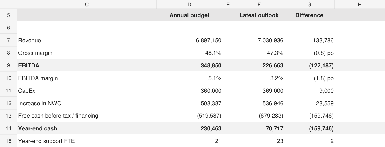
Higher sales do not guarantee higher profit.

The latest outlook has more revenue than the budget, but higher costs and support payroll reduce EBITDA. Cash falls further because the business also needs to fund working capital and equipment.

Revenue vs. budget+1.9%$133,786 increase

EBITDA vs. budget−35.0%$122,187 decrease

Outlook year-end cash$70,717From $750,000 opening cash

Source: Dashboard!D7:G14. Full-year outlook combines January–June simulated actuals and July–December forecast.

01 / Purpose & assumptions

The business case

Northstar Components represents a manufacturer with one product group. The project tests whether its sales plan can cover production costs, support staff and other operating expenses, while leaving enough cash for equipment and day-to-day operations.

I used a manufacturing setting because units, material cost and production cost give the financial model a clear operating basis. The aim is to explain why the forecast changes, rather than only report a final profit number.

Inputs behind the plan

Driver	Budget assumption	Why it matters
Annual units	51,090	Monthly sales volumes drive revenue and variable costs.
Selling price	$135 per unit	Multiplied by units to calculate revenue.
Material / conversion cost	$45 / $25 per unit	Conversion includes direct production labor and variable factory costs.
Support staff	20 opening FTE	Hires and exits roll forward into payroll.
Salary / employer burden	$84,000 / 20%	Average paid FTE × monthly salary × burden factor.
Other operating expenses	$55,000/month + 3.5% of sales	Fixed and variable selling, general and administrative costs (SG&A).
Receivable / inventory / payable days	36 / 42 / 28	Estimate how much cash is tied up in operations.

Source: Assumptions!D8:D18; Headcount!D8. FTE means full-time equivalent.

How the forecast is updated

January–June uses fixed observations on the Actuals sheet. July–December assumes 2% more volume, 1% higher prices, 3% higher material cost and 2% higher fixed SG&A than budget. The salary-change input is 0%; hiring is modeled separately in Headcount.

Source: Assumptions!L22:Q26; Forecast!F6:Q6.

02 / Budget & outlook

Revenue improves. Margins tighten.

Budget revenue is 51,090 units × $135 = $6,897,150. The full-year outlook reaches $7,030,936, but support payroll rises by $111,342 and COGS rises by $126,749. These increases explain why EBITDA declines even with higher sales.

2027 full-year comparison · USD unless stated
Measure	Budget	Latest outlook	Outlook − budget
Revenue	$6,897,150	$7,030,936	+$133,786
Cost of goods sold	$3,576,300	$3,703,049	+$126,749
Gross profit	$3,320,850	$3,327,888	+$7,038
Gross margin	48.1%	47.3%	-0.82 pp
Support payroll	$2,070,600	$2,181,942	+$111,342
SG&A	$901,400	$919,283	+$17,883
EBITDA	$348,850	$226,663	−$122,187
EBITDA margin	5.1%	3.2%	-1.83 pp
Support staff at year-end (FTE)	21	23	+2

Source: Budget and Forecast, annual totals in column D; Headcount!D12 and D27. A positive cost difference means higher expense. Margin changes are percentage points (pp).

Actual workbook dashboard showing budget and latest outlook, including revenue, EBITDA and ending cash. — Dashboard excerpt from the attached workbook. Select the image for the full-size view.

03 / Variance analysis

Why first-half EBITDA missed budget

For January–June, revenue is $32,477 above plan, while EBITDA is $64,545 below plan. A driver bridge separates the changes in volume, price, unit cost, payroll and SG&A.

January–June EBITDA bridge · USD
Driver	Profit impact
Budget EBITDA	$218,476
Unit volume effect	−$3,445
Selling price effect	+$39,632
Raw-material unit cost effect	−$39,667
Conversion unit cost effect	−$21,786
Support payroll effect	−$31,542
SG&A effect	−$7,737
Simulated actual EBITDA	$153,932

Source: Variance!D18:D26. Rounded rows may differ by $1 from the total.

Reading the bridge

The $39,632 selling-price benefit is almost fully offset by the $39,667 increase from material unit costs. Conversion costs and support payroll add further pressure.

This is why I would review material costs and hiring alongside sales. Reporting revenue alone would miss the deterioration in operating profit.

The SG&A line contains its full variance, including variable selling expenses. The price line is a revenue effect before those expenses.

04 / Cash planning

Positive EBITDA, negative cash flow

The outlook produces $226,663 of EBITDA, but $536,946 of additional net working capital and $369,000 of CapEx use more cash than the operation generates.

$226,663 − $536,946 − $369,000 = −$679,283EBITDA − increase in net working capital − CapEx = cash flow before tax and financing

Outlook cash balance · USD

Source: Assumptions!D30 and Cash flow!F29:Q29. The line begins with the opening balance before January.

View monthly cash balances

Period	Ending cash
Opening	$750,000
Jan	$307,191
Feb	$297,450
Mar	$235,588
Apr	$275,594
May	$227,024
Jun	$272,793
Jul	$279,164
Aug	$277,102
Sep	$247,419
Oct	$194,729
Nov	$129,776
Dec	$70,717

The large January cash outflow partly reflects the opening working-capital balances being below the first month’s modeled run rate. I would validate those opening balances before using the model for a real cash decision.

Conclusion: positive EBITDA does not mean the company can fund all of its investment needs. Receivable collection, inventory levels and the timing of equipment spending all matter.

05 / Scenario & sensitivity

What if materials cost 8% more and volume falls 5%?

The Scenario sheet applies this stress to the original annual budget. Selling price, support payroll and fixed SG&A remain unchanged. Conversion cost and variable SG&A decrease with activity.

Budget EBITDA$348,850

Stressed EBITDA$20,149

Change−94.2%

EBITDA falls by $328,700. Material spending still rises by $59,775: the combination of 5% lower volume and 8% higher unit cost is 0.95 × 1.08 = 1.026, or a 2.6% increase in material spending.

The workbook also includes a sensitivity grid for volume changes from −10% to +5% and material-cost changes from 0% to +12%. At −5% volume and +12% material cost, annual EBITDA becomes negative at −$67,214.

Source: Scenario!D7:D9, F12:H20 and F25:I29. This test measures annual budget EBITDA, not a separate cash forecast.

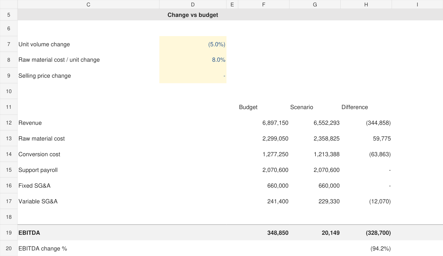
Show the scenario calculation from Excel

Scenario worksheet with input changes and budget versus stress EBITDA calculations. — Scenario worksheet excerpt. Select the image to enlarge.

Conclusion: the budget’s 5.1% EBITDA margin leaves limited room for adverse changes. A volume decline reduces contribution while payroll and fixed SG&A remain in place.

06 / Excel methods

How the worksheets connect

Assumptions and Actuals feed Budget, Forecast and Headcount. Working capital and CapEx then feed Cash flow. Dashboard, Variance and Scenario summarize the results. Checks reviews the calculations without feeding operating formulas.

Revenue

Budget!F10 = F8*F9

January: 4,150 units × $135 = $560,250.

Cost of goods sold

Budget!F16 = SUM(F14:F15)

Materials ($186,750) + conversion costs ($103,750) = $290,500. Direct production labor is already included in conversion cost.

Support payroll

Headcount!F16 = F13*F14/'Assumptions'!$D$35*(1+F15)

Average FTE × annual salary ÷ 12 × (1 + burden). January: 20 × $84,000 ÷ 12 × 1.20 = $168,000. Averaging opening and closing FTE approximates mid-month hiring.

EBITDA

Budget!F27 = F17-F21-F25

Gross profit − support payroll − SG&A. CapEx is a cash outflow, not an EBITDA expense.

Working capital

'Working capital'!F15 = F8*F11/'Assumptions'!$D$34

Receivables = monthly revenue × receivable days ÷ 30. Inventory and payables use COGS as a simplified run rate. Net working capital = receivables + inventory − payables.

Cash rollforward

'Cash flow'!F29 = F28+F26

Opening cash + cash flow = closing cash. The next month starts with the previous month’s closing balance.

Techniques demonstrated

Cross-sheet references, absolute and mixed cell references, monthly rollforwards, SUM, AVERAGE, IF, ABS, ROUND and SUMPRODUCT. Annual margins divide annual profit by annual revenue, rather than averaging monthly percentages. Ending balances use December rather than the sum of 12 months.

The workbook has 12 reconciliation checks covering revenue, EBITDA, payroll, working capital, cash and the scenario. All show OK in the reviewed copy. These confirm internal consistency; they do not establish that the assumptions are realistic.

Source: Checks!C7:F18. Formula examples are taken directly from the downloadable workbook.

Model scope and limitations

One product group and 30-day planning months.
Conversion costs are modeled per unit; this simplifies production cost behavior.
Inventory and supplier payables use COGS-based estimates rather than a purchasing ledger.
Payroll and SG&A are paid in the month incurred.
No tax, interest, financing, depreciation or net-income schedule. Cash flow is before tax and financing.

07 / Takeaways

What I take from this project

Explain the change, not just the total.
The variance bridge gives a reason for the EBITDA miss. Higher selling prices help, but material costs, conversion costs and payroll use up that benefit.
Keep profit and cash separate.
Equipment spending and increases in working capital reduce cash without being deducted in the same way from EBITDA.
Make assumptions easy to find.
Separating inputs from formulas makes it easier to change a driver, trace the effect and explain the result.

Questions I would investigate next

Can pricing offset material inflation? Does the additional support hiring match the operating need? Can receivables be collected sooner, or equipment purchases scheduled differently? These are follow-up questions from the model, not claims of savings already achieved.

Review the project

Open the Excel model

Start with Dashboard, then follow Assumptions → Budget / Forecast → Variance → Cash flow. Use Scenario!D7:D9 to test the annual stress.

The workbook download is the file supplied for this portfolio. The figures on this page are a fixed snapshot and will not update when you edit your downloaded copy.

Download workbook ↓Back to top